Understanding Recurrent Neural Networks

In my last post, we used our micro-framework to learn about and create a Convolutional Neural Network. It was super cool, so check it out if you haven’t already. Now, in my final post for this tutorial series, we’ll be similarly learning about and building Recurrent Neural Networks (RNNs). RNNs are neural networks that are fantastic at time-dependent tasks, especially tasks that have to do with time series as an input. RNNs can serially process each time step of the series in order to build a semantic representation of the whole time series, one step at a time.

In this post, we will understand the math and intuition behind RNNs. We will build out RNN features in our micro-framework, use them to create an RNN, and train the RNN on a sequence classification task.

Recurrent Layers

A recurrent layer is a layer which has a temporal connection to itself. This connect allows the layer to model time-dependent functions. Let’s say our data is a time series of vectors which vary over every time step. The recurrent layer consists of a cell which takes as inputs the current time step and the last cell output. The cell does some computation on the inputs to produce the output.

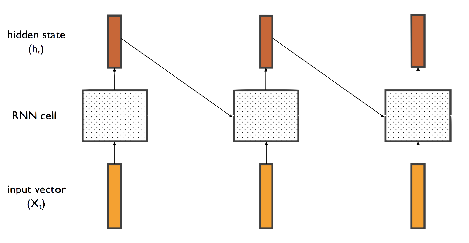
Note that there is only one RNN cell, but it has been repeated multiple times for sake of simplicity. At each time step, the cell produces an output, the hidden state of the cell. If our input time series has time step vectors with D elements, and we chose our hidden state vector’s size to be H, then a time series of dimensions N x T x D will have an output of N x T x H, where N is the batch size and T is the amount of time steps in each time series. We can use this output tensor to learn insights about the time series.

Vanilla RNN Cells

The simplest way to combine the two inputs (the current time step input as well as the previous cell output) to produce the next output is to multiply each by a weight and add them together–with a non-linearity on the output, of course. Thus, we have our very simple vanilla RNN cell equation:

That’s it! This is pretty easy to implement, so let’s get right into it. First, the initializer:

class VanillaRNN(Layer):
    def __init__(self, input_dim, hidden_dim):
        super(VanillaRNN, self).__init__()
        self.params['Wh'] = np.random.randn(hidden_dim, hidden_dim)
        self.params['Wx'] = np.random.randn(input_dim, hidden_dim)
        self.params['b'], self.h0 = np.zeros(hidden_dim), np.zeros((1, hidden_dim))
        self.D, self.H = input_dim, hidden_dim

Next, the forward pass. Since the RNN cell is reused for every step in the time series, we create a step function which executes at each time step. The forward function, then, calls the step functions at every time step:

    def forward_step(self, input, prev_h):
        cell = np.matmul(prev_h, self.params['Wh']) + np.matmul(input, self.params['Wx']) + self.params['b']
        next_h = np.tanh(cell)

        self.cache['caches'].append((input, prev_h, next_h))

        return next_h

    def forward(self, input):
        N, T, _ = input.shape
        H = self.H
        self.cache['caches'] = []
        h = np.zeros((N, T, H))

        h_cur = self.h0
        for t in range(T):
            h_cur= self.forward_step(input[:, t, :], h_cur)
            h[:, t, :] = h_cur

        return h

We return a tensor which is a time series of all of the cell outputs at each time step.

Now, the backward pass, which we similarly break down into a step function and a series function. One note on this step: because the RNN cell is reused for every time step, the gradient must be accumulated over all time steps–that is, instead of the gradient being set, we must start with zero and added to at ever time step of the backward pass. Here’s how the backward pass looks:

    def backward_step(self, dnext_h, cache):
        input, prev_h, next_h = cache
        dcell = (1 - next_h ** 2) * dnext_h

        dx = np.matmul(dcell, self.params['Wx'].T)
        dprev_h = np.matmul(dcell, self.params['Wh'].T)

        dWx = np.matmul(input.T, dcell)
        dWh = np.matmul(prev_h.T, dcell)

        db = np.sum(dcell, axis=0)

        return dx, dprev_h, dWx, dWh, db

    def backward(self, dout):
        N, T, _ = dout.shape
        D, H = self.D, self.H
        caches = self.cache['caches']
        dx, dh0, dWx, dWh, db = np.zeros((N, T, D)), np.zeros((N, H)), np.zeros((D, H)), np.zeros((H, H)), np.zeros(H)

        for t in range(T - 1, -1, -1):
            dx[:, t, :], dh0, dWx_cur, dWh_cur, db_cur = self.backward_step(dout[:, t, :] + dh0, caches[t])
            dWx += dWx_cur
            dWh += dWh_cur
            db += db_cur

        self.grads['Wx'], self.grads['Wh'], self.grads['b'] = dWx, dWh, db

        return dx

We loop backwards through the incoming gradient’s time steps, pass them through our backward step function, and accumulate the gradients through the backward unrolling. Note that we add the derivative of the previous hidden state to the gradient on each output hidden state at time step. This is because the previous hidden state is passed in as an input in the forward pass and hence must be accounted for in the backward pass, and it’s most convenient to do this computation in the series function rather than the step function.

That’s it! Now we can use vanilla RNN cells in our code.

Sequence Classification

Let’s put our vanilla RNN cells to use on a sequence classification task! Let’s have a time series of 2 elements, where the label is a 0 if the difference between the two is <= 0, and a 1 otherwise. Let’s create a quick loader class to create such a dataset:

class RecurrentTestLoader(Loader):
    def __init__(self, batch_size):
        super(RecurrentTestLoader, self).__init__(batch_size)

        train, validation, test = self.load_data()
        self.train_set, self.train_labels = train
        self.validation_set, self.validation_labels = validation
        self.test_set, self.test_labels = test

    def load_data(self, path=None):
        timeseries = np.random.randint(1, 10, size=(16000, 2, 1))

        targets = timeseries[:, 0] - timeseries[:, 1]
        neg, pos = np.where(targets <= 0), np.where(targets > 0)
        targets[neg], targets[pos] = 0, 1

        timeseries_train = timeseries[:8000, :]
        timeseries_val = timeseries[8000:12000, :]
        timeseries_test = timeseries[12000:16000, :]

        targets_train = targets[:8000]
        targets_val = targets[8000:12000]
        targets_test = targets[12000:16000]

        return (timeseries_train, targets_train.astype(np.int32)), (timeseries_val, targets_val.astype(np.int32)), (timeseries_test, targets_test.astype(np.int32))

Let’s initialize our loader and network:

loader = RecurrentTestLoader(16)

layers = [VanillaRNN(1, 4),
          ReLU(),
          Flatten(),
          Linear(8, 2)]
loss = SoftmaxCrossEntropy()
recurrent_network = Sequential(layers, loss, 1e-3, regularization=L2(0.01))

Notice that we use a Flatten layer to turn the time series of hidden state outputs into a 2-dimensional tensor that can be passed into the final Linear layer. Finally, let’s train our model!

for i in range(10000):
    batch, labels = loader.get_batch()

    pred, loss = recurrent_network.train(batch, labels)

    if (i + 1) % 100 == 0:
        accuracy = eval_accuracy(pred, labels)
        print("Training Accuracy: %f" % accuracy)

    if (i + 1) % 500 == 0:
        accuracy = eval_accuracy(recurrent_network.eval(loader.validation_set), loader.validation_labels)
        print("Validation Accuracy: %f \n" % accuracy)

accuracy = eval_accuracy(recurrent_network.eval(loader.test_set), loader.test_labels)
print("Test Accuracy: %f \n" % accuracy)

That’s it! We have used our Vanilla RNN cell on a fairly simple time-dependent problem that illustrates its purpose and functionality. However, there’s a problem–it doesn’t work! Because we repeatedly multiply the same cell weight with its derivative, the gradient will either explode or vanish. This is (rather fittingly) called the exploding/vanishing gradient problem. To solve this problem, a new type of cell was invented: Long Short-Term Memory (LSTM) cells.

LSTM Cells

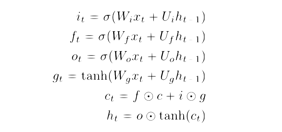
An LSTM cell, similar to a vanilla RNN cell, uses both the current input and its previous output to produce its current output. However, what’s interesting about LSTM cells is that it actually produces two outputs, both of which it uses in its next unrolling: the hidden state and the cell state. The cell state is only modified through the use of controlled gates, as defined by these equations:

The input gate (i_t) is a gate which is directly multiplied with the previous cell state, thereby deciding how much new information is added to the cell state. The forget gate (f_t) is is a gate that decides how much of the previous cell state is “forgotten”. The input gate is multiplied by a gate (g_t) which decides what is added to the cell state, and is then added to the cell state with some information forgotten by the forget gate. This sum is the new cell state. Finally, the output gate (o_t) is a gate which is multiplied with the new cell state and decide how much is exposed as the next hidden state. Here’s how all of that looks as a diagram:

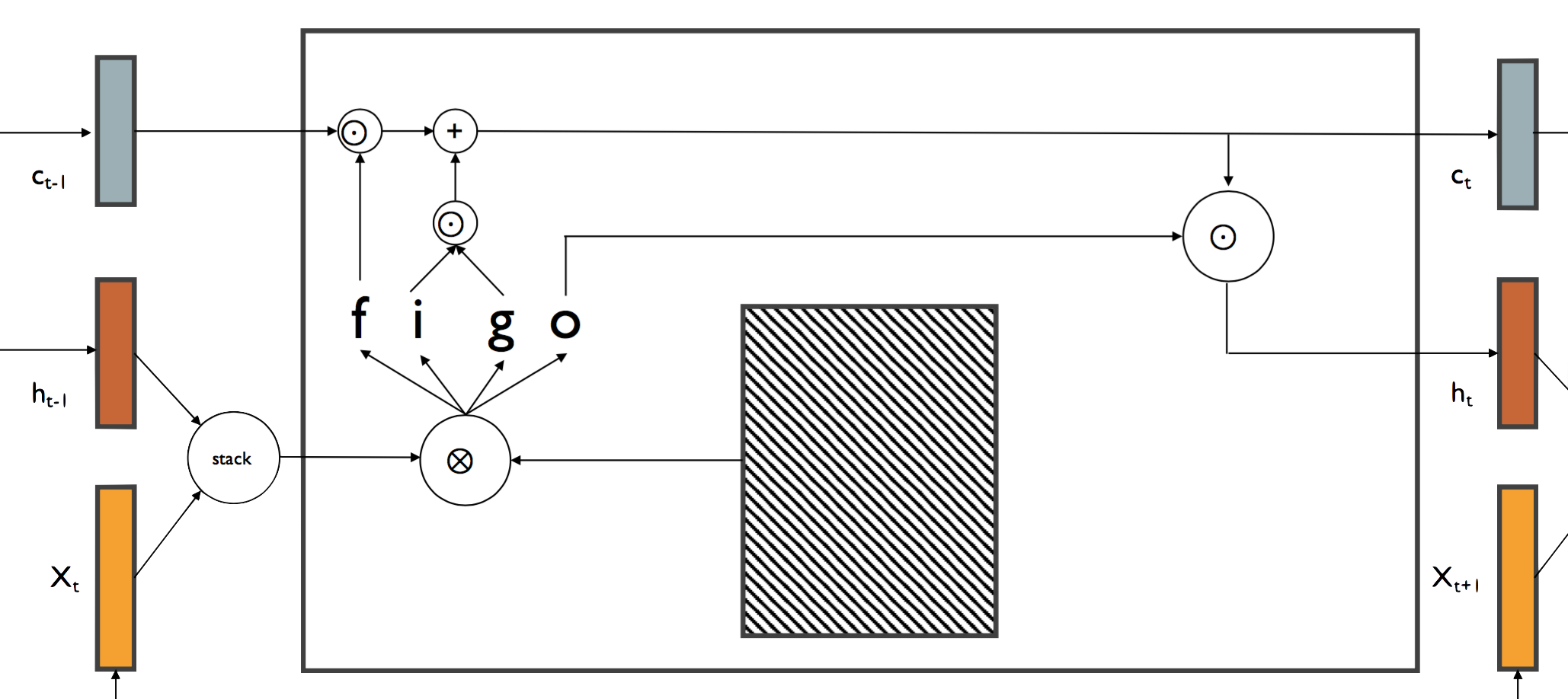
The benefit of the LSTM cell is that there is a direct connection between the cells previous state and its current state, meaning that gradients can more easily backpropagate through the cells without vanishing. Because only the forget and input gates directly interact with the cell state, long-term dependencies can more easily persist through many unrollings.

The cell state can be thought of in another way as well. The cell state at time t can be thought of as an encoded representation of the time series by time t. The fact that it takes the previous output as an input means that each time step input is used to continuously update the internal representation of the time series. So, by the end, the output is the encoded representation of the entire time series. For example, if we feed the cell a sentence, one word at a time, the output of the final cell computation is a vector representation of the sentence’s semantic meaning. This final state can be used in addition to the hidden state sequence to learn interesting insights.

Let’s start implementing an LSTM cell! We can make the implementation easier on ourselves if we think of all the inputs getting concatenated and being multiplied by one huge weight; we then split the output of this computation into the individual gates. Here’s the initializer:

class LSTM(Layer):
    def __init__(self, input_dim, hidden_dim):
        super(LSTM, self).__init__()
        self.params['W'], self.params['b'] = np.random.randn(input_dim + hidden_dim, 4 * hidden_dim), np.zeros(4 * hidden_dim)
        self.h0 = np.zeros((1, hidden_dim))
        self.D, self.H = input_dim, hidden_dim

Now forward the forward pass:

def forward_step(self, input, prev_h, prev_c):
        N, _ = prev_h.shape
        H = self.H
        input = np.concatenate((input, prev_h), axis=1)
        gates = np.matmul(input, self.params['W']) + self.params['b']

        i = utils.sigmoid(gates[:, 0:H])
        f = utils.sigmoid(gates[:, H:2 * H])
        o = utils.sigmoid(gates[:, 2 * H:3 * H])
        g = np.tanh(gates[:, 3 * H:4 * H])

        next_c = f * prev_c + i * g
        next_h = o * np.tanh(next_c)

        self.cache['caches'].append((input, prev_c, i, f, o, g, next_c, next_h))

        return next_h, next_c

    def forward(self, input):
        N, T, _ = input.shape
        D, H = self.D, self.H
        self.cache['caches'] = []

        h = np.zeros((N, T, H))
        h_prev = self.h0
        c = np.zeros((N, H))
        for t in range(T):
            x_curr = input[:, t, :]
            h_prev, c = self.forward_step(x_curr, h_prev, c)
            h[:, t, :] = h_prev

        return h

Here’s the backward pass:

def backward_step(self, dnext_h, dnext_c, cache):
        input, prev_c, i, f, o, g, next_c, next_h = cache
        D = self.D

        dtanh_next_c = dnext_h * o
        dcell = (1 - next_h ** 2) * dnext_h
        dnext_c += dtanh_next_c * dcell

        dc = dnext_c * f

        di = dnext_c * g
        df = dnext_c * prev_c
        do = dnext_h * np.tanh(next_c)
        dg = dnext_c * i

        dgates1 = di * i * (1 - i)
        dgates2 = df * f * (1 - f)
        dgates3 = do * o * (1 - o)
        dgates4 = dg * (1 - g ** 2)
        dgates = np.concatenate((dgates1, dgates2, dgates3, dgates4), axis=1)

        db = np.sum(dgates, axis=0)

        dW = np.matmul(input.T, dgates)

        dinput = np.matmul(dgates, self.params['W'].T)
        dx = dinput[:, :D]
        dh = dinput[:, D:]

        return dx, dh, dc, dW, db

    def backward(self, dout):
        N, T, _ = dout.shape
        D, H = self.D, self.H
        dx, dh0, dW, db, dc = np.zeros((N, T, D)), np.zeros((N, H)), np.zeros((D + H, 4 * H)), np.zeros(4 * H), np.zeros((N, H))
        caches = self.cache['caches']


        for t in range(T - 1, -1, -1):
            dx[:, t, :], dh0, dc, dW_cur, db_cur = self.backward_step(dout[:, t, :] + dh0, dc, caches[t])
            dW += dW_cur
            db += db_cur

        self.grads['W'], self.grads['b'] = dW, db

        return dx

We can use the diagram from above as a pseudo-graph to break down the backward pass. First, we notice that the next cell state branches into two outputs: the outputted next cell state and the next hidden state. The next cell state’s gradient is given to us as an incoming gradient; we must also account for the gradient on the next cell state due to the next hidden state. We do this by multiplying the next hidden state by the output gate (which the next cell state is multiplied with in the forward pass), take the derivative of the tanh function with respect to the next hidden state, multiply these values together, and add it to our incoming next cell state gradient. The gradient on the cell state is then the gradient on the next cell state multiplied with the forget gate. This was all done by simply tracing all the lines from the outputs to the cell state input.

The gradients on the gates is fairly straightforward: the gradient on the forget gate is the gradient on next cell state times the previous cell state, the gradient on the input gate is the gradient on the next cell state times g, the gradient on g is the gradient on the next cell state multiplied by the input gate, and the gradient on the output gate is the gradient on the next hidden state times the tanh of the next cell state. (again, this is all easy to see by tracing all the lines from all outputs to these gates). We take the derivative of the tanh or sigmoid functions with respect to each gate (note: these are left out of the diagram graph) and concatenate them together to get the final gradient on all gates. This can easily be used to get the gradients on the weight, bias, and input of the layer, in a manner similar to the backward pass of a linear layer. One last thing: we split the input into the gradients on time step vector and the previous cell state, as those were stacked together in the forward pass.

Now, we can replace the VanillaRNN layer with our LSTM to get much better performance on our sequence classification problem. Sweet!

Next Steps

Recurrent networks are incredibly powerful tools which can be applied to some incredible problems. For example, in language translation, a source sentence is encoded by an RNN into an intermediate representation of the semantic meaning of the sentence, and then that representation is used by another RNN to decode it into a target language. Here is a paper on using RNNs for machine translation, and here is a PyTorch tutorial on the subject.

Another cool application of RNNs: a convolutional network pretrained on image classification is used to turn an image into an intermediate representation, which is then used as the initial hidden state of an LSTM cell to caption the picture. Here is the original paper on topic, and here is a Torch (not PyTorch) implementation of the latest iteration of the paper.

One last plug: one of my close friends made a hilarious RNN project which is trained on Trump’s Tweet corpus to produce “new” Trump tweets. Check out the code here.

I really hope you’ve enjoyed this tutorial series and found it to be educational and useful! If you have any questions, you can reach out to me at @ShubhangDesai on Twitter. There’s a whole world of deep learning, the surface of which we’ve barely scratched–go and explore it! Happy learning!