Understanding Convolutional Neural Networks

In my last post, we learned about some advanced neural network topics and built them into our NN micro-framework. Now, we put that advanced framework to use to understand Convolutional Neural Networks (CNNs). CNNs are neural networks which are mostly employed on vision tasks–that is, problems that have to do with pictures. The benefit of using a CNN over a fully-connected network on images is that CNNs preserve spatial relationships and can gain insights into the visual structure of the input picture.

In this post, we will explore the math and intuition behind CNNs. We will also add to our micro-framework a Convolution layer and use it to create a simple, 3-hidden layer CNN on an image classification task.

Convolutional Layers

A convolutional layer is a layer which computes dot products over an input feature map to create an output feature map. A feature map is a 3-dimensional tensor in which two of the dimensions can be thought of as spatial width and height. The convolutional layer has one shared weight, known as a filter which is smaller than the feature map itself and is “slid” over the map to compute the dot product. As the filter slides over the input, it maps the dot product results to an output feature map, which can also be thought of as an image and can hence be fed as input into another convolutional layer.

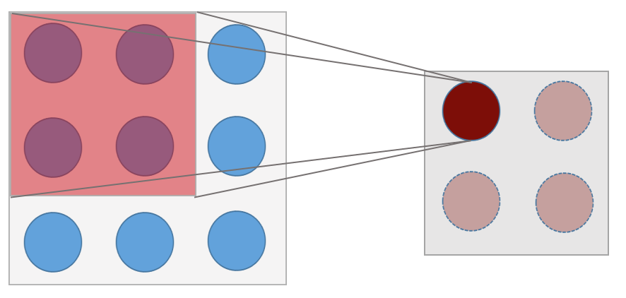
Shown above is a 3x3 image with a 2x2 convolutional filter being slid over it. At the current position the filter is at, the dot product between the image elements and the filter is taken and the output is mapped to the first element of the output feature map, so on and so forth. The filter then slides over 1 pixel and produces the second output feature map element. The size of the final output is 2x2.

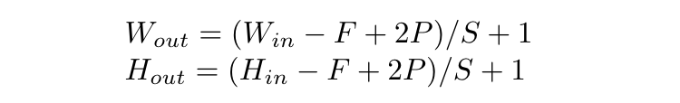
The amount that the filter is moved on each slide is known as the stride. The size of the filter itself is known as the kernel size or spatial extent. Each of the dot products is computed depth-wise, so each filter outputs a feature map of depth 1. We can have multiple filters in a convolutional layer so that its output has a larger depth. We can surround the border of the input with white pixels, known as padding, so that the output is larger and the filter can compute dot product over more of the input. All of these hyperparameters mean that the size of the output feature map is dependent on many variables. For example, if the input is 4x4, the kernel size is 2x2, and the stride is 2 with a padding of 0, the output is 2x2. Here is the equation to figure out what the output size is given the various hyperparameters:

So that’s the math behind convolutional layers. But why do we want to do this? The fact that we use only one shared weight every time we “slide” over the whole image reflects the assumptions that “knowledge” that can be applied to one piece of the image can also be applied to another. For example, if there’s something that looks like an ear in a picture of a dog in one part of the image, we want to reuse the weight that understands it on the second ear in the same picture. In addition, the fact that we don’t just stretch the input feature map into one long column vector means that spatial information is preserved in the layer, which is crucial when we are doing vision tasks. This all means that convolutional layers are very powerful when we want our network to learn about images.

Code Implementation

Let’s add to our Layers file a Convolutional layer. The initializer should take the layer hyperparameters and initialize the filters, which we store in one huge 4-dimensional matrix. We also save the filter amount and kernel size as properties for convenient use in the forward function:

class Convolutional(Layer):
    def __init__(self, channels, num_filters, kernel_size, stride=1, pad=0):
        super(Convolutional, self).__init__()
        self.params["W"] = np.random.randn(num_filters, channels, kernel_size, kernel_size) * 0.01
        self.params["b"] = np.zeros(num_filters)

        self.stride = stride
        self.pad = pad

        self.F = num_filters
        self.HH, self.WW = kernel_size, kernel_size

The input to the forward pass should be a 3-dimensional tensor, as should the output. Here’s the code for the forward function:

  def forward(self, input):
        N, C, H, W = input.shape
        F, HH, WW = self.F, self.HH, self.WW
        stride, pad = self.stride, self.pad

        H_prime = 1 + (H + 2 * pad - HH) / stride
        W_prime = 1 + (W + 2 * pad - WW) / stride
        assert H_prime.is_integer() and W_prime.is_integer(), 'Invalid filter dimension'
        H_prime, W_prime = int(H_prime), int(W_prime)

        out = np.zeros((N, F, H_prime, W_prime))
        filters = self.params["W"].reshape(F, C * HH * WW)
        x_pad = np.pad(input, pad_width=((0, 0), (0, 0), (pad, pad), (pad, pad)), mode='constant', constant_values=0)

        for i in range(H_prime):
            h_start = i * stride
            h_end = h_start + HH
            for j in range(W_prime):
                w_start = j * stride
                w_end = w_start + WW

                kernel = x_pad[:, :, h_start:h_end, w_start:w_end]
                kernel = kernel.reshape(N, C * HH * WW)

                conv = np.matmul(kernel, filters.T) + self.params["b"]
                out[:, :, i, j] = conv

        self.cache["input"] = input
        return out

This function is pretty dense so let’s break it down. First we compute the output feature map dimensions using the above equations. Then, we instantiate the output feature map as a zero tensor, reshape the filters to a convenient shape for computation, and pad the input. Then we slide the filter over the input’s spatial dimension using two loops over the dimensions. The code in the inner loop takes the piece of the input that we are computing the dot product with, reshape it to convenient shape, perform the dot product, and store the result in the appropriate mapping location in the output feature map.

As you might imagine, the backwards pass for this operation is fairly complicated:

  def backward(self, dout):
        input = self.cache["input"]
        stride, pad = self.stride, self.pad
        N, C, H, W = input.shape
        F, HH, WW = self.F, self.HH, self.WW
        _, _, H_prime, W_prime = dout.shape

        H_pad, W_pad = H + 2 * pad, W + 2 * pad
        dx = np.zeros((N, C, H + 2 * pad, W + 2 * pad))
        dW = np.zeros_like(self.params["W"])
        db = np.sum(dout, axis=(0, 2, 3))
        filters = self.params["W"].reshape(F, C * HH * WW)
        x_pad = np.pad(input, pad_width=((0, 0), (0, 0), (pad, pad), (pad, pad)), mode='constant', constant_values=0)

        for i in range(H_prime):
            h_start = i * stride
            h_end = h_start + HH
            for j in range(W_prime):
                w_start = j * stride
                w_end = w_start + WW

                piece = dout[:, :, i, j]
                x_piece = x_pad[:, :, h_start:h_end, w_start:w_end].reshape(N, C * HH * WW)
                dx_piece = np.matmul(piece, filters)
                dW_piece = np.matmul(piece.T, x_piece)

                dx[:, :, h_start:h_end, w_start:w_end] += dx_piece.reshape(N, C, HH, WW)
                dW += dW_piece.reshape(F, C, HH, WW)

        dx = dx[:, :, pad:H_pad - pad, pad:W_pad - pad]
        self.grads["W"], self.grads["b"] = dW, db

        return dx

This is a monstrosity, so we’ll break it down again. The first thing we do is instantiate some useful variables that we’ll be using later on. We initialize the gradients on the input and filters as zero matrices, and we are able to directly compute the gradient on the bias by summing the incoming gradient across some dimensions. Notice that the gradient matrix on the input is initialized with the padded dimensions of the input, not the true input dimensions; this is important, as you’ll see soon. We once again loop over the spatial dimensions, but this time of the incoming gradient.

This is where it gets interesting: we take specific slices of the incoming gradient and the input to the forward pass. Notice that that specific slice of the incoming gradient is from the same position in forward pass output feature map that was the result of a matrix multiplication between the filters and the input feature map slice that we just took. This means that we can now treat the incoming gradient piece as the output of a simple matrix multiplication between the input feature map piece and the filters and do backpropagation as expected: simply multiply the incoming gradient piece with the filters to get the gradient on the input, and multiply the incoming gradient piece with the input feature map piece to get the gradient on the filters. However, instead of setting the gradients to those values, we add it to the previously initialized matrices, as the gradients are aggregated over the whole loop over the spatial dimensions. One final step: we trim off the padded elements of the input gradient that were needed to do the aggregations to get the final gradient on the input at that layer. We save the gradients on the weight and the bias, and we’re finally ready to return the gradient on the input. Phew!

Image Classification

Let’s take our Convolutional layer for a run by building a CNN that we train on an image classification task. Image classification is the task of giving an algorithm a picture and having it determine what it is out of a known list of possible classes. We will use the small but useful CIFAR-10 dataset to do this. The dataset has 10 classes (airplane, automobile, bird, cat, deer, dog, frog, horse, ship, truck) and can be downloaded here.

Data Loading

Before we start making the model, let’s create a Loader class which can load and sample the dataset. We will use this class to give us a batch of data during train time. Here’s the initializer:

class Loader(object):
    def __init__(self, batch_size, path="datasets/cifar-10-batches-py"):
        super(Loader, self).__init__()
        self.batch_size = batch_size

        train, validation, test = self.load_data(path)
        self.train_set, self.train_labels = train
        self.validation_set, self.validation_labels = validation
        self.test_set, self.test_labels = test

        self.train_set, mean, std = self.preprocess(self.train_set)
        self.validation_set = (self.validation_set - mean)/std
        self.test_test = (self.test_set - mean)/std

We want to 1) load the data and 2) preprocess it. Preprocessing is fitting the training data to a Gaussian distribution, and using the training statistics to “normalize” the validation and test sets. Here’s the code to load the data:

    def load_data(self, path):
        train_set, train_labels = np.zeros((0, 3, 32, 32)), np.zeros((0))
        validation_set, validation_labels = None, None
        test_set, test_labels = None, None

        files = [path + "/data_batch_%d" % (i+1) for i in range(5)]
        files.append(path + "/test_batch")
        for file in files:
            with open(file, 'rb') as fo:
                dict = pickle.load(fo, encoding='bytes')

            batch_set = dict[b"data"].reshape(10000, 3, 32, 32)
            batch_labels = np.array(dict[b"labels"]).reshape(10000)

            if "5" in file:
                validation_set, validation_labels = batch_set, batch_labels
            elif "test" in file:
                test_set, test_labels = batch_set, batch_labels
            else:
                train_set = np.concatenate((train_set, batch_set))
                train_labels = np.concatenate((train_labels, batch_labels))

        return (train_set, train_labels.astype(np.int32)), (validation_set, validation_labels.astype(np.int32)), (test_set, test_labels.astype(np.int32))

And here’s the code to preprocess the data:

    def preprocess(self, set):
        mean, std = np.mean(set, axis=0), np.std(set, axis=0)
        set -= mean
        set /= std
        return set, mean, std

Finally let’s add a function to give us a batch of data:

    def get_batch(self):
        indeces = np.random.choice(self.train_set.shape[0], self.batch_size, replace=False)
        batch = np.array([self.train_set[i] for i in indeces])
        labels = np.array([self.train_labels[i] for i in indeces])

        return batch, labels

Building and Training a CNN

One more step before we build and train a network: we need to make a super simple Layer which flattens the final feature map from a 4-dimensional tensor into a vector:

class Flatten(Layer):
    def __init__(self):
        super(Flatten, self).__init__()

    def forward(self, input):
        self.cache["shape"] = input.shape

        return input.reshape(input.shape[0], -1)

    def backward(self, dout):
        return dout.reshape(self.cache["shape"])

Now let’s build a 3-hidden-layer CNN that takes as input the 28x28 pixels images and outputs a 1x10 vector of class probabilities. We will use Softmax-Cross-Entropy as our loss function. Here’s the code to do that:

loader = Loader(batch_size=16)

layers = [Convolutional(3, 5, 6, stride=2),
          Convolutional(5, 7, 6, stride=2),
          Convolutional(7, 10, 4),
          Flatten()]
loss = SoftmaxCrossEntropyLoss
conv_network = Network(layers, loss, 1e-3)

Finally, we train our network!

for i in range(10000):
    batch, labels = loader.get_batch()

    pred, loss = conv_network.train(batch, labels)

    if (i + 1) % 100 == 0:
        accuracy = eval_accuracy(pred, labels)
        print("Training Accuracy: %f" % accuracy)

    if (i + 1) % 500 == 0:
        accuracy = eval_accuracy(conv_network.eval(loader.validation_set), loader.validation_labels)
        print("Validation Accuracy: %f \n" % accuracy)

accuracy = eval_accuracy(conv_network.eval(loader.test_set), loader.test_labels)
print("Test Accuracy: %f \n" % accuracy)

Unfortunately, this does not yield great accuracy. In order to do better on this task, we’ll have to add more complex layers to the network.

Advanced Layers

Let’s code up some more layers that will make our convolutional network more advanced and (hopefully) accurate.

Spatial Batch Normalization

As you may recall from the last post, batch normalization is a good way to fit a layer’s output to a Gaussian distribution, reducing overfitting by your network. We want to employ this ability in our convolutional network. However, our BatchNorm layer expects a 2-dimensional input, while our feature map is 4-dimensional. We remedy this by simply reshaping the tensor before and after the BatchNorm forward and backward passes. Because we want to normalize over the spatial dimensions, the first dimension is the width times height times batch size, and the second dimension is necessarily the number of channels. Here’s the code:

class BatchNorm2d(BatchNorm):
    def __init__(self, dim, epsilon=1e-5, momentum=0.9):
        super(BatchNorm2d, self).__init__(dim, epsilon, momentum)

    def forward(self, input):
        N, C, H, W = input.shape
        output = super(BatchNorm2d, self).forward(input.reshape(N * H * W, C))
        return output.reshape((N, C, H, W))

    def backward(self, dout):
        N, C, H, W = dout.shape
        dx = super(BatchNorm2d, self).backward(dout.reshape(N * H * W, C))
        return dx.reshape((N, C, H, W))

Finally, add BatchNorm2d to the Network class’s diff tuple. Now we can add a batch normalization layer to convolutional networks.

Max Pooling

Max pooling is a layer which reduces the dimensionality of the a feature map. Similar to a convolution, the max pooling layer slides over the feature map; however, instead of computing the dot product of the kernel with a weight, it simply takes the maximum value in that kernel and sends it to the output feature map. That’s it! This prevents overfitting as well, as it does reduces dependence on specific neurons, and also reduces computational cost by reducing the dimensionality without the need of additional parameters. Here’s the code:

class MaxPooling(Layer):
    def __init__(self, kernel_size, stride=1, pad=0):
        super(MaxPooling, self).__init__()
        self.stride = stride
        self.pad = pad

        self.HH, self.WW = kernel_size, kernel_size

    def forward(self, input):
        N, C, H, W = input.shape
        HH, WW, stride = self.HH, self.WW, self.stride

        H_prime = (H - HH) / stride + 1
        W_prime = (W - WW) / stride + 1
        out = np.zeros((N, C, H_prime, W_prime))

        if not H_prime.is_integer() or not W_prime.is_integer():
            raise Exception('Invalid filter dimension')

        H_prime, W_prime = int(H_prime), int(W_prime)

        for i in range(H_prime):
            h_start = i * stride
            h_end = h_start + HH
            for j in range(W_prime):
                w_start = j * stride
                w_end = w_start + WW

                kernel = input[:, :, h_start:h_end, w_start:w_end]
                kernel = kernel.reshape(N, C, HH * WW)
                max = np.max(kernel, axis=2)

                out[:, :, i, j] = max

        self.cache['input'] = input
        return out

    def backward(self, dout):
        input = self.cache['input']
        N, C, H, W = input.shape
        HH, WW, stride = self.HH, self.WW, self.stride

        H_prime = int((H - HH) / stride + 1)
        W_prime = int((W - WW) / stride + 1)
        dx = np.zeros_like(input)

        for i in range(H_prime):
            h_start = i * stride
            h_end = h_start + HH
            for j in range(W_prime):
                w_start = j * stride
                w_end = w_start + WW

                max = dout[:, :, i, j]

                kernel = input[:, :, h_start:h_end, w_start:w_end]
                kernel = kernel.reshape(N, C, HH * WW)
                indeces = np.argmax(kernel, axis=2)
                grads = np.zeros_like(kernel)
                for n in range(N):
                    for c in range(C):
                        grads[n, c, indeces[n, c]] = max[n, c]

                dx[:, :, h_start:h_end, w_start:w_end] += grads.reshape(N, C, HH, WW)

        return dx

This looks long, but it is almost identical to the Convolutional layer, so I won’t spend time explaining it. We can now add max pooling to our convolutional network.

Advanced Network

Now that we have some cool layers implemented, let’s take another shot at image classification. Let’s change our Layers list to and run the training regement again:

layers = [Convolutional(3, 5, 4, stride=2),
          ReLU(),
          BatchNorm2d(5),
          MaxPooling(2, stride=1),

          Convolutional(5, 7, 4, stride=2),
          ReLU(),
          BatchNorm2d(7),
          MaxPooling(2, stride=1),

          Convolutional(7, 10, 5, stride=1),
          Flatten()]

Sweet! We just created a convolutional neural network which is able to predict the class of a given CIFAR-10 image with about 50% validation accuracy! This may not sound too great, but considering that there are 10 classes, and that this is a simplistic network architecture with very few parameters, that’s not too bad!

You may be wondering: how does a simple 3-hidden-layer architecture do as well as it does on this task? The reason is that each layer can be thought to learn more and more complex insights about the original input. The first layer, for example, detects edges; the next assembles those edges into shapes; and the last layer assembles shapes into higher-level concepts, such as ears, wings, or wheels. This way of thinking about the architecture has roots in research by Hubel & Wiesel which showed that the image-processing in a cat’s brain occurs in a similar hierarchical pattern as the one described above.

Next Steps

We used the CIFAR-10 Dataset to test out our model. There are many other publicly available image datasets like CIFAR-10 specifically made for image classification. One example is the MS-COCO dataset, a large dataset with pictures and accompanying annotations and captions. ImageNet a huge dataset with hundres of clases. The creators of the dataset hold a yearly competition to see who can build a network that achieves the highest accuracy on the set.

We employed a classic–and simple–CNN architecture in our exercise. Some really crazy CNN architectures have been created over the last few years. For example, VGG-Net is recently-developed CNN that is 19 layers deep; Google’s well-known Inception network consists of Inception modules that split and concatenate feature maps through many non-sequential convolutions; and ResNet is an extremely deep (as in 152-layer) CNN which employs Residual Blocks that can learn to “ignore” certain convolutional layers completely. Check out some of the linked papers to learn more about recent advances in computer vision!

Next week, we’ll be using our framework to learn about and create a Recurrent Neural Network for time-dependent problems, such as language translation or audio analysis. Check back next week for that. Happy learning!