A Comprehensive Look into Neural Artistic Style Transfer

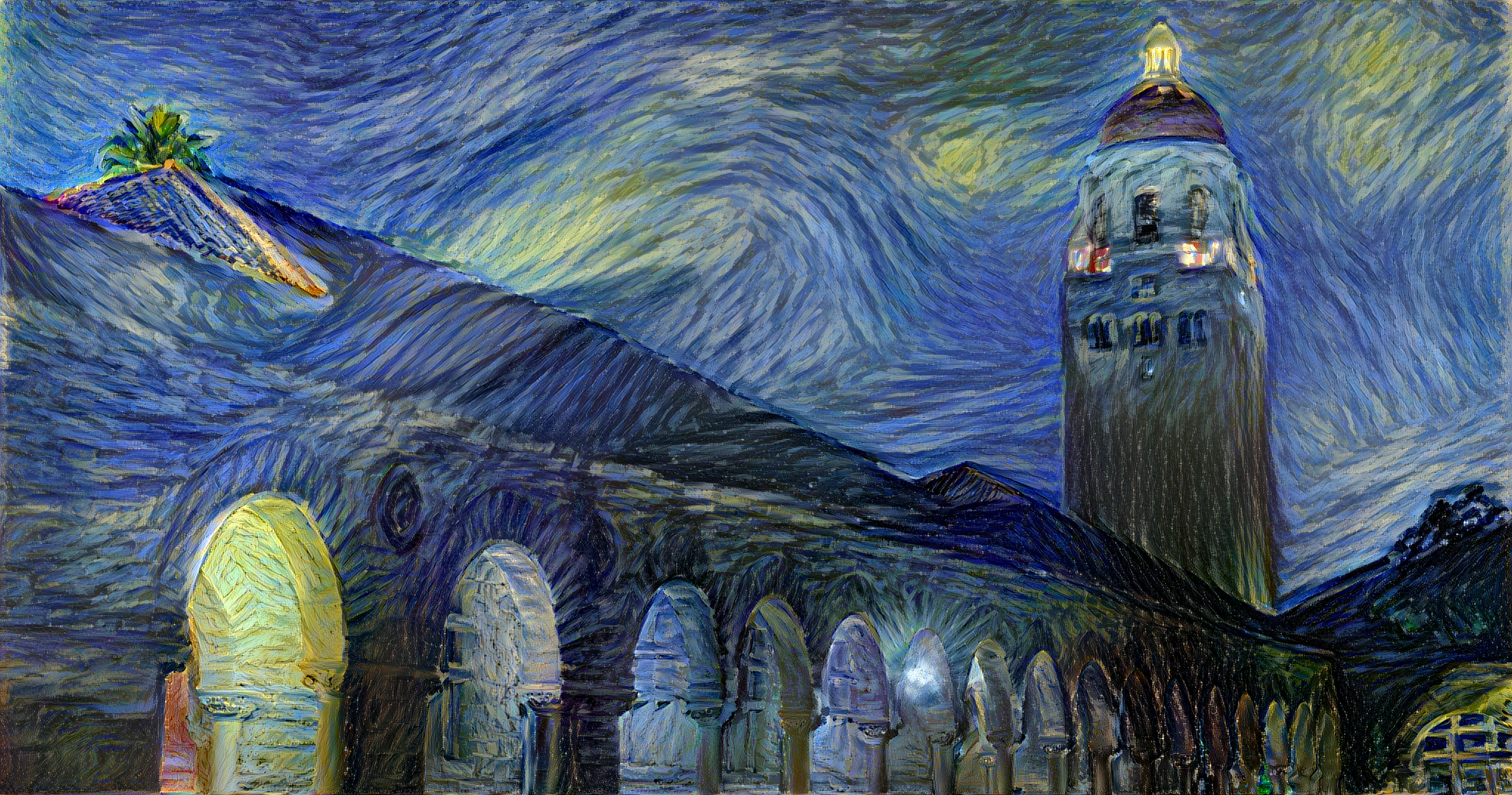
This past year, I took Stanford’s CS 231n course on Convolutional Neural Networks. My final project for the course dealt with a super cool concept called neural style transfer, in which the style of a piece of artwork is transferred onto a picture. Here’s a classic example–a picture of Hoover Tower at Stanford, in the style of The Starry Night:

There is a long and rich history of the buildup to neural style transfer, but we’ll focus specifically on this sphere in this article. The first published paper on neural style transfer used an optimization technique–that is, starting off with a random noise image and making it more and more desirable with every “training” iteration of the neural network. This technique has been covered in quite a few tutorials around the web. However, the technique of a subsequent paper, which is what really made neural style transfer blow up, has not been covered as thoroughly. This technique is feedforward–train a network to do the stylizations for a given painting beforehand so that it can produce stylized images instantly.

In this tutorial, we will cover both techniques–the intuitions and math behind how they work, and how the second builds off the first. We will also cover the next step in cutting-edge research, as explored by me in my CS 231n project, as well as research teams at Cornell and Google. By the end, you will be able to train your own networks to produce beautiful pieces of art!

Optimization Method

In this method, we do not use a neural network in a “true” sense. That is, we aren’t training a network to do anything. We are simply taking advantage of backpropagation to minimize two defined loss values. The tensor which we backpropagate into is the stylized image we wish to achieve–which we call the pastiche from here on out. We also have as inputs the artwork whose style we we to transfer, known as the style image, and the picture that we want to transfer the style onto, known as the content image.

The pastiche is initialized to be random noise. It, along with the content and style images, are then passed through several layers of a network that is pretrained on image classification. We use the outputs of various intermediate layers to compute two types of losses: style loss and content loss–that is, how close is the pastiche to the style image in style, and how close is the pastiche to the content image in content. Those losses are then minimized by directly changing our pastiche image. By the end of a few iterations, the pastiche image now has the style of the style image and the content of the content image–or, said differently, a stylized version of the original content image.

Losses

Before we dive into the math and intuition behind the losses, let’s address a concern you may have. You may be wondering why we use the outputs of intermediate layers of a pretrained image classification network to compute our style and content losses. This is because, for a network to be able to do image classification, it has to understand the image. So, between taking the image as input and outputting its guess at what it is, it’s doing transformations to turn the image pixels into an internal understanding of the content of the image.

We can interpret these internal understandings as intermediate semantic representations of the initial image and use those representations to “compare” the content of two images. In other words, if we pass two images of cats through an image classification network, even if the initial images look the very different, in many internal layers, their representations will be very close in raw value. This is the content loss–pass both the pastiche image and the content image through some layers of an image classification network and find the Euclidean distance between the intermediate representations of those images. Here’s the equation for content loss:

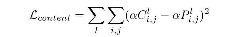
The summation notation looks makes the concept look harder than it really is. Basically, we make a list of layers at which we want to compute content loss. We pass the content and pastiches images through the network until one of the layers in the list, take the output of that layer, square the difference between corresponding each value in the output, and sum them all up. We do this for every layer in the list, and sum those up. One thing to note, though: we multiply each of the representations by some value alpha before finding their differences and squaring it.

The style loss is very similar, except instead of comparing the raw outputs of the style and pastiche images at various layers, we compare the Gram matrices of the outputs. A Gram matrix is a matrix which results from multiplying a matrix with the transpose of itself:

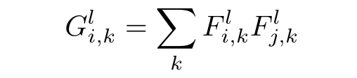
Because every column is multiplied with every row in the matrix, we can think of the spatial information that was contained in the original representations to have been “distributed”. The Gram matrix instead contains non-localized information about the image, such as texture, shapes, and weights–style! Now that we have defined the Gram matrix as having information about style, we can find the Euclidean distance between the Gram matrices of the intermediate representations of the pastiche and style image to find how similar they are in style:

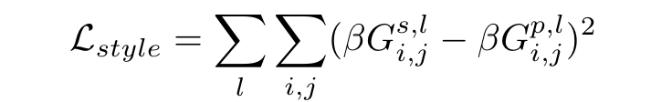
Now that we have the content loss–which contains information on how close the pastiche is in content to the content image–and the style loss–which contains information on how close the pastiche is in style to the style image–we can add them together to get the total loss. We then backpropagate through the network to reduce this loss by getting a gradient on the pastiche image and iteratively changing it to make it look more and more like a stylized content image. This is all described in more rigorous detail in the original paper on the topic by Gatys et al.

Implementation

Now that we know how it works, let build it. First, let’s implement the Gram matrix layer:

import torch
import torch.nn as nn

class GramMatrix(nn.Module):
    def forward(self, input):
        a, b, c, d = input.size()
        features = input.view(a * b, c * d)
        G = torch.mm(features, features.t())

        return G.div(a * b * c * d)

Now, let’s define our network. Let’s create a class with an initializer that sets some important variables:

import torch.optim as optim
import torchvision.models as models

from modules.GramMatrix import *

class StyleCNN(object):
    def __init__(self, style, content, pastiche):
        super(StyleCNN, self).__init__()

        self.style = style
        self.content = content
        self.pastiche = nn.Parameter(pastiche.data)

        self.content_layers = ['conv_4']
        self.style_layers = ['conv_1', 'conv_2', 'conv_3', 'conv_4', 'conv_5']
        self.content_weight = 1
        self.style_weight = 1000

        self.loss_network = models.vgg19(pretrained=True)

        self.gram = GramMatrix()
        self.loss = nn.MSELoss()
        self.optimizer = optim.LBFGS([self.pastiche])

        self.use_cuda = torch.cuda.is_available()
        if self.use_cuda:
            self.loss_network.cuda()
            self.gram.cuda()

The variables which we initialize are: the style, content, and pastiches images; the layers at which we compute content and style loss, as well as the alpha and beta weights we multiply the representations by; the pretrained network that we use to get the intermediate representations (we use VGG-19); the Gram matrix computation; the loss computation we do (as MSE is the same as Euclidean distance); and the optimizer we use. We also want to make use of a GPU if we have on on our machine.

Now for the network’s “training” regime. We pass the images through the network one layer at a time. We check to see if it is a layer at which we do a content or style loss computation. If it is, we compute the appropriate loss at that layer. Finally, we add the content and style losses together and call backward on that loss, and take an update step. Here’s how all that looks:

    def train(self):
      def closure():
        self.optimizer.zero_grad()

        pastiche = self.pastiche.clone()
        pastiche.data.clamp_(0, 1)
        content = self.content.clone()
        style = self.style.clone()

        content_loss = 0
        style_loss = 0

        i = 1
        not_inplace = lambda layer: nn.ReLU(inplace=False) if isinstance(layer, nn.ReLU) else layer
        for layer in list(self.loss_network.features):
            layer = not_inplace(layer)
            if self.use_cuda:
                layer.cuda()

            pastiche, content, style = layer.forward(pastiche), layer.forward(content), layer.forward(style)

            if isinstance(layer, nn.Conv2d):
                name = "conv_" + str(i)

                if name in self.content_layers:
                    content_loss += self.loss(pastiche * self.content_weight, content.detach() * self.content_weight)
                if name in self.style_layers:
                    pastiche_g, style_g = self.gram.forward(pastiche), self.gram.forward(style)
                    style_loss += self.loss(pastiche_g * self.style_weight, style_g.detach() * self.style_weight)

            if isinstance(layer, nn.ReLU):
                i += 1

        total_loss = content_loss + style_loss
        total_loss.backward()

        return total_loss

    self.optimizer.step(closure)

    return self.pastiche

(To use the LBGFS optimizer, it is necessary to pass into the step function a closure function which “reevaluates the model and returns the loss”; we don’t need to do that with any other optimizer…go figure)

One more step before we can start transferring some style: we need to write up a couple of convenience functions:

import torchvision.transforms as transforms
from torch.autograd import Variable

from PIL import Image

import scipy.misc

imsize = 256

loader = transforms.Compose([
  transforms.Scale(imsize),
  transforms.ToTensor()])

unloader = transforms.ToPILImage()

def image_loader(image_name):
  image = Image.open(image_name)
  image = Variable(loader(image))
  image = image.unsqueeze(0)
  return image

def save_image(input, path):
  image = input.data.clone().cpu()
  image = image.view(3, imsize, imsize)
  image = unloader(image)
  scipy.misc.imsave(path, image)

The image_loader function opens an image at a path and loads it as a PyTorch variable of size imsize; the save_image function turns the pastiches image, which is a PyTorch variable, into the appropriate PIL format to save it to file.

Now, to produce beautiful art. First, let’s import some stuff, load our images, and put them onto the GPU if we have one:

import torch.utils.data
import torchvision.datasets as datasets

from StyleCNN import *
from utils import *

# CUDA Configurations
dtype = torch.cuda.FloatTensor if torch.cuda.is_available() else torch.FloatTensor

# Content and style
style = image_loader("styles/starry_night.jpg").type(dtype)
content = image_loader("contents/dancing.jpg").type(dtype)
pastiche = image_loader("contents/dancing.jpg").type(dtype)
pastiche.data = torch.randn(input.data.size()).type(dtype)

num_epochs = 31

Finally, let’s define and call our training loop to turn our initially random pastiche into an incredible piece of art:

def main():
    style_cnn = StyleCNN(style, content, pastiche)

    for i in range(num_epochs):
        pastiche = style_cnn.train()

        if i % 10 == 0:
            print("Iteration: %d" % (i))

            path = "outputs/%d.png" % (i)
            pastiche.data.clamp_(0, 1)
            save_image(pastiche, path)

main()

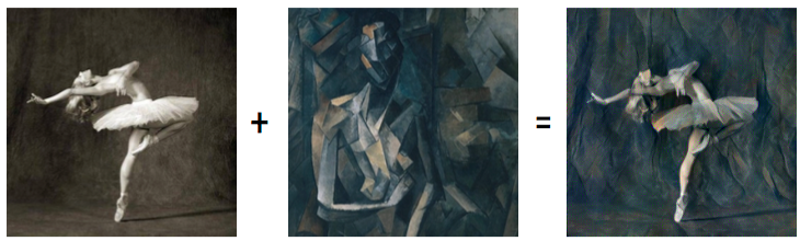
And that’s it! We have used an optimization method to generate a stylized version of a content image. You can now render any image into the style of any painting–albeit slowly, as the optimization process takes time. Here’s an example that I made from our code: a dancer in the style of a Picasso:

Feedforward Method

Why does the previous method take so much time? Why do we have to wait for an optimization loop to generate a pretty picture? Can’t we tell a network, “Hey, learn the style of Starry Night so well that I can give you any picture and you’ll turn it into a Starry Night-ified version of the picture instantly”? As a matter of fact, we can!

Essentially, we have an untrained Image Transformation Network which transforms the content image into its best guess at an appealing pastiche image. We then use this as the pastiche image which, along with the content and style images, is passed through the pretrained image classification network (now called the Loss Network) to compute our content and style losses. Finally, to minimize the loss, we backpropagate into the parameters of the Image Transormation Network, not directly into the pastiche image. We do this with a ton of random content image examples, thereby training the Image Transformation Network how to transform any given picture into the style of some predefined artwork.

Implementation

We now need to add an Image Transformation Network to our now multi-stage network architecture, and make sure that the optimizer is set to optimize the parameters of the ITN. We will be using the architecture from Johnson et al. for our ITN. Replace the last 8 lines of the StyleCNN initializer with this code:

        self.transform_network = nn.Sequential(nn.ReflectionPad2d(40),
                                               nn.Conv2d(3, 32, 9, stride=1, padding=4),
                                               nn.Conv2d(32, 64, 3, stride=2, padding=1),
                                               nn.Conv2d(64, 128, 3, stride=2, padding=1),
                                               nn.Conv2d(128, 128, 3, stride=1, padding=0),
                                               nn.Conv2d(128, 128, 3, stride=1, padding=0),
                                               nn.Conv2d(128, 128, 3, stride=1, padding=0),
                                               nn.Conv2d(128, 128, 3, stride=1, padding=0),
                                               nn.Conv2d(128, 128, 3, stride=1, padding=0),
                                               nn.Conv2d(128, 128, 3, stride=1, padding=0),
                                               nn.Conv2d(128, 128, 3, stride=1, padding=0),
                                               nn.Conv2d(128, 128, 3, stride=1, padding=0),
                                               nn.Conv2d(128, 128, 3, stride=1, padding=0),
                                               nn.Conv2d(128, 128, 3, stride=1, padding=0),
                                               nn.ConvTranspose2d(128, 64, 3, stride=2, padding=1, output_padding=1),
                                               nn.ConvTranspose2d(64, 32, 3, stride=2, padding=1, output_padding=1),
                                               nn.Conv2d(32, 3, 9, stride=1, padding=4),
                                              )
    self.gram = GramMatrix()
    self.loss = nn.MSELoss()
    self.optimizer = optim.Adam(self.transform_network.parameters(), lr=1e-3)

    self.use_cuda = torch.cuda.is_available()
    if self.use_cuda:
    self.loss_network.cuda()
        self.gram.cuda()                    

Also, since we now want our training regime to accept a content image batch as training examples, we can remove the content image as an input to the initializer. Our training regime accepts a content image batch, transforms it into pastiche images, computes losses as done above, and calls backward on the final loss to update the ITN parameters. Here’s all that in code:

    def train(self, content):
        self.optimizer.zero_grad()

        content = content.clone()
        style = self.style.clone()
        pastiche = self.transformation_network.forward(content)

        content_loss = 0
        style_loss = 0

        i = 1
        not_inplace = lambda layer: nn.ReLU(inplace=False) if isinstance(layer, nn.ReLU) else layer
        for layer in list(self.loss_network.features):
            layer = not_inplace(layer)
            if self.use_cuda:
                layer.cuda()

            pastiche, content, style = layer.forward(pastiche), layer.forward(content), layer.forward(style)

            if isinstance(layer, nn.Conv2d):
                name = "conv_" + str(i)

                if name in self.content_layers:
                    content_loss += self.loss(pastiche * self.content_weight, content.detach() * self.content_weight)
                if name in self.style_layers:
                    pastiche_g, style_g = self.gram.forward(pastiche), self.gram.forward(style)
                    style_loss += self.loss(pastiche_g * self.style_weight, style_g.detach() * self.style_weight)

            if isinstance(layer, nn.ReLU):
                i += 1

        total_loss = content_loss + style_loss
        total_loss.backward()

        self.optimizer.step()

        return self.pastiche

Awesome! Let’s change our save_image function to be able to save not just one image, but a batch of images:

def save_images(input, paths):
    N = input.size()[0]
    images = input.data.clone().cpu()
    for n in range(N):
        image = images[n]
        image = image.view(3, imsize, imsize)
        image = unloader(image)
        scipy.misc.imsave(paths[n], image)

One more order of business. We need to have available to us a dataset of content images as training examples to be passed into our network at every training iteration. We will use the Microsoft COCO dataset for this. You have to install and set up the COCO API before you can do anything with it in PyTorch. The API can be download from source here. After downloading it, install it by running setup.py.

Once you’ve completed those steps, add these imports:

import torch.utils.data
import torchvision.datasets as datasets

Finally, we replace our main function with this code:

  num_epochs = 3
  N = 4

  def main():
    style_cnn = StyleCNN(style)

    # Contents
    coco = datasets.ImageFolder(root='data/contents', transform=loader)
    content_loader = torch.utils.data.DataLoader(coco, batch_size=N, shuffle=True, **kwargs)

    for epoch in range(num_epochs):
        for i, content_batch in enumerate(content_loader):
          iteration = epoch * i + i
          content_loss, style_loss, pastiches = style_cnn.train(content_batch, style_batch)

          if i % 10 == 0:
              print("Iteration: %d" % (iteration))
              print("Content loss: %f" % (content_loss.data[0]))
              print("Style loss: %f" % (style_loss.data[0]))

          if i % 500 == 0:
              path = "outputs/%d_" % (iteration)
              paths = [path + str(n) + ".png" for n in range(N)]
              save_images(pastiches, paths)

              path = "outputs/content_%d_" % (iteration)
              paths = [path + str(n) + ".png" for n in range(N)]
              save_images(content_batch, paths)
              style_cnn.save()

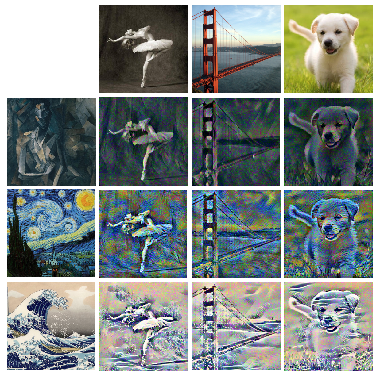
Woo! Now we can train a network to transform any image into a stylized version of it, based on the style of our prepicked image. That is awesome! In case you were wondering, this technology is exactly how apps like Prisma work. Here are some examples from three feedforward networks trained on three different paintings:

Arbitrary Style Transfer

You may have noticed that, although our feedforward implementation can produce stylized pastiches instantly, it can only do so for one given style image. Would it be possible to train a network which can take, in addition to any content image, any style image and produce a pastiche from those two images? In other words, can be make a truly arbitrary neural style transfer network?

As it so happens, a very cool finding in this problem suggested that it is possible. A few years ago, it was found that the Instance Normalization layers in the Image Transformation Networks were the only important layers to represent style. In other words, if we keep all Convolutional parameters the same and learn only new Instance Normalization parameters, we can represent completely different styles in just one network. Here’s the paper with that finding. This suggests that we can take advantage of Instance Norm layers by using in those layers parameters that are specific to each style.

The first attempt to do this was from a team at Cornell. Their solution was using Adaptive Instance Normalization, in which an encoder-decoder architecture was used to generate the Instance Norm parameters from the style images. Here is the paper on that. This has fairly high success.

The next attempt at arbitrary style transfer was my own project, in which I use a secondary Normalization Network to transform the style image into Instance Normalization parameters to be used by the Image Transformation Network, learning the parameters in both the Normalization Network and the ITN all at once. Here’s my paper on that. While this method was also theoretically successful, it was only able to demonstrate success on small set of style images and not truly arbitrary.

The latest attempt at achieving arbitrary style transfer was from a team at Google Brain. They used a method almost identical to the one described above, except that they use a pretrained Inception network to transform the style images into Instance Norm parameters instead of using and untrained network and training it, along with the ITN, end-to-end. This method saw wild success and produced beautiful results, achieving true arbitrary neural style transfer. Here is the awesome paper on that.

While I was unable to fully solve the problem, I felt honored to have been able to participate in the research conversation and be on the cutting-edge of such as exciting project. It was thrilling to Google finally solve the problem with such an elegant and beautiful solution.

Next Steps

There’s quite a bit of literature on this problem, so some great next steps would be to skim through them. I linked the papers throughout the article, but I thought I’d post them all in one place too:

• Here is the original paper on neural style transfer, which proposed the optimization process
• Here is the paper on feedforward style transfer; its supplementary materials contain the architecture that we used in our code.
• If you were wondering what Instance Normalization even is, here is the paper describing it.
• Here is the Cornell paper on Adaptive Instance Norm
• Here is my paper on end-to-end arbitrary style transfer network training
• Here is the Google paper which achieved arbitrary style transfer

Hope you found this exciting application of neural networks to be as fascinating and fun as I do. Happy learning!