Advanced Exploration into Neural Networks

In my last post, we built a modular neural network micro-framework that will help us learn more about NNs. Although we were going to start building a Convolutional Neural Network in this tutorial, I thought it might be useful to first learn a little bit more about more advanced aspects of neural networks and build them out in our framework. That way, when we start making CNNs and RNNs soon, we will have more of the necessary infrastructure built out already. By the end of this tutorial, we will learn about activation functions, regularization, batch normalization, and dropout. We will also build out these features in our micro-framework.

Activation Functions

An activation function is a function that we apply to the output of a neural network layer to control how much of the output is exposed to the next layer. This is implemented as a layer that comes between two layers. Once a layer completes its computation and produces an output, we pass each of the elements of the output through the activation layer, a scalar-valued function, to produce the “activated” neurons as output. A good way to think of this is by extending the “brain” analogy: akin to these contrived activation functions, our neural cells have activation functions between its axon terminals and dendrites that squash, amplify, or even nullify certain signals as an electric impulse passes through it.

The purpose of these functions is to introduce non-linearities in our network. Imagine a 1-hidden-layer fully-connected network, as we built before. This is simply a linear function: f(x) = Wx + b. Now imagine a 2-hidden-layer fully-connected network with no activation function in between: f(x) = W₂(W₁x + b₁) + b₂. Without the non-linear activation function, there is nothing stopping this function from collapsing into a simple linear function, just like a 1-hidden-layer neural network, only with more complex notation. It is non-linear activation functions that truly allow neural networks to model non-trivial problems and learn interesting insights.

Some popular activation functions include tanh function, sigmoid function, and ReLU (Rectified Linear Units), the last of which is the most popular.

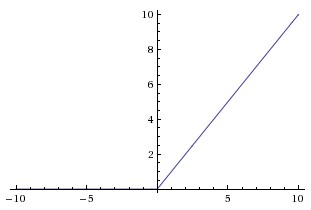
Above is the graph of the ReLU function. It is super simple: keep the value the same if it is non-negative, and make it zero if it is negative. That’s it! Even though it is simple, ReLU has been empirically shown to perform very well on real-world problems.

Enough talking, let’s code! Let’s create our ReLU function:

class ReLU(Layer):
    def __init__(self):
        super(ReLU, self).__init__()

    def forward(self, input):
        mask = input >= 0
        self.cache["mask"] = mask
        input[~mask] = 0
        return input

    def backward(self, dout):
        mask = self.cache["mask"]
        dout = dout * mask
        return dout

The forward pass is fairly simple: we create a mask which is all the places in the output where the value is 0 or higher (i.e. positive). Then, we make all the values in the output which are not the mask (i.e. negative) 0 and return it. We also cache the mask. In the backward pass, we multiply the incoming gradient with the mask, because all the values which were made negative in the forward pass had no effect on the final output and hence those positions must be turned to 0 in the backward pass. Easy! Now we can add ReLU layers to our neural networks.

Regularization

Our objective in training a neural network is to find “good values” for the parameters in the network such that it solves the problem given to it as accurately as possible. However, there’s never just one good value for any parameter; in fact, there’s infinitely many answers which may work. However, while some of those answer may yield high training accuracy, they may fail to generalize and hence will perform poorly in the real world. This is called overfitting.

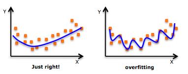
Above is an example of overfitting: the curve of the right fits the points almost perfectly, but is horrible at generalizing, while the one of the curve on the left fits the points well and can generalize too! We want to prevent our network from overfitting, because, after all, we don’t care about training accuracy–we want our network to make accurate predictions in the real world.

We can use regularization to prevent overfitting. Regularization is penalizing parameters which overfit the data, hence forcing the network to produce generalizations. One of the simplest methods of regularization is L2 Regularization, in which we simply add the square of the Frobenius Norm of each parameter (scaled by some small value α) to the loss value. This way, when we minimize the loss value, we also make sure that the parameter values stay small in magnitude:

Once again, this is a computation just like any other in the network, and hence must have a forward and backward pass. The derivative of the L2 Regularization function is fairly simple:

Essentially, this means that we add 2α times the previous value of the parameter to the gradient, and use that to update the parameter.

Although the math is very easy, adding this to our code will be fairly involved. Let’s start simple and code up a Regularization superclass:

class Regularization(object):
    def __init__(self, weight):
        super(Regularization, self).__init__()
        self.weight = weight

    def forward(self, param):
        raise NotImplementedError

    def backward(self, param):
        raise NotImplementedError

And now for the L2 class:

class L2(Regularization):
    def __init__(self, weight):
        super(L2, self).__init__(weight)

    def forward(self, param):
        return self.weight * np.sum(param * param)

    def backward(self, param):
        return 2 * self.weight * param

That was pretty easy. Now let’s add the ability to regularize parameters in our Network class. First, let’s modify the Network initializer so that it can accept a regularizer:

def __init__(self, layers, loss, lr, regularization=None):
        super(Network, self).__init__()
        self.layers = layers
        self.loss = loss
        self.lr = lr
        self.regularization = regularization

Now for the tough part. We need to strategically place code in our network’s forward passes so that the regularization occurs. Let’s break it up into two parts: the forward pass and the backward pass. In the Sequential object’s train function, we loop through the layers and call their forward functions. Now, we want to slightly modify that so that the regularization loss is added to the total loss:

l = 0
  for layer in layers:
    input = layer.forward(input)
    if regularization is not None:
      for _, param in layer.params.items():
        l += regularization.forward(param)

l += loss.forward(input, target)

Not too bad. This reflects the addition of the regularization in the loss value. However, the important part is making the regularization reflect in the gradient updates. Currently, in we loop through the reversed layers list and call their forward functions. We want to similarly modify this to change the gradients that are used to update the parameters:

for layer in reversed(layers):
  dout = layer.backward(dout)

  for param, grad in layer.grads.items():
    if regularization is not None:
      grad += regularization.backward(layer.params[param])
    layer.params[param] -= self.lr * grad

And that’s it! Now, we can pass the L2 object into the network to make sure that the parameters of the network’s layers are not overfitting to the training data!

Batch Normalization

There are other ways to prevent overfitting than just regularization your network’s weights. We can add special layers which “regularize” the network. One such layer is a batch normalization layer. In this layer, the input is basically turned into a Gaussian distribution (zero-mean and one std.), which is a useful way for the subsequent layer to compare features, as opposed to the arbitrarily scaled and shifted distribution produced as the output of the layer before the BN layer. However, BN layers to something very useful in addition to that: they scale and shift the normalized output by some learned parameters, known as gamma and beta, respectively. In theory, they could learn to scale by the standard deviation and shift by the mean, and “un-normalize” the data, if it turns out that a Gaussian distribution is not as useful. The gamma and beta of BN layers allow for precise control over the “Gaussian-ness” of the layer’s output. Here’s the equation for batch normalization:

There’s also one more interesting thing about BN layers: they behave differently at train-time and at test-time. During train-time, we want to normalize the batch and hence want to use the statistics of the batch itself. However, during test-time, we want to normalize using statistics of the whole dataset. Because computing these statistics is difficult (and perhaps impossible, as the test-time input that the network receives in the real-world may be completely new data), we instead keep a running mean and running variance that we update with every training iteration, and use those statistics during test-time.

Enough explanation, let’s start coding our BN layer. First, the initializer:

def BatchNorm(Layer):
    def __init__(self, dim, epsilon=1e-5, momentum=0.9):
        super(BatchNorm, self).__init__()
        self.params['gamma'] = np.ones(dim)
        self.params['beta'] = np.zeros(dim)

        self.running_mean, self.running_var = np.zeros(dim), np.zeros(dim)
        self.epsilon, self.momentum = epsilon, momentum

        self.mode = "train"

The epsilon is used for numerical stability during the forward pass, and the momentum is used to update the running statistics. Now for the forward pass:

    def forward(self, input):
        gamma, beta = self.params['gamma'], self.params['beta']
        running_mean, running_var = self.running_mean, self.running_var
        epsilon, momentum = self.epsilon, self.momentum

        if self.mode == 'train':
            mean, var = np.mean(input, axis=0), np.var(input, axis=0)
            norm = (input - mean) / np.sqrt(var + epsilon)
            output = gamma * norm + beta

            running_mean = momentum * running_mean + (1 - momentum) * mean
            running_var = momentum * running_var + (1 - momentum) * var

            self.running_mean, self.running_var = running_mean, running_var
            self.cache['input'], self.cache['norm'], self.cache['mean'], self.cache['var'] = input, norm, mean, var
        else:
            norm = (input - running_mean) / np.sqrt(running_var)
            output = gamma * norm + beta

        return output

In the forward pass, we first initialize some important variables and check whether we are training or testing. If we are training, we compute the batch statistics, normalize the input, and scale and shift the normalized input. We also update our running statistics and cache some variables we’ll need in the backward pass. If we are testing, we simply use the running statistics to normalize the input, and then scale and shift the normalized input.

Finally, the backward pass:

  def backward(self, dout):
      input, norm, mean, var = self.cache['input'], self.cache['norm'], self.cache['mean'], self.cache['var']
      gamma, beta = self.gamma, self.beta
      epsilon = self.epsilon
      N, _ = dout.shape

      self.grads['beta'] = np.sum(dout, axis=0)
      self.grads['gamma'] = np.sum(dout * norm, axis=0)

      dshift1 = 1 / (np.sqrt(var + epsilon)) * dout * gamma

      dshift2 = np.sum((input - mean) * dout * gamma, axis=0)
      dshift2 = (-1 / (var + epsilon)) * dshift2
      dshift2 = (0.5 / np.sqrt(var + epsilon)) * dshift2
      dshift2 = (2 * (input - mean) / N) * dshift2

      dshift = dshift1 + dshift2

      dx1 = dshift
      dx2 = -1 / N * np.sum(dshift, axis=0)
      dx = dx1 + dx2

      return dx

The backward pass is certainly a beast, and its derivation is way outside of the scope of this post. You can read a very in-depth explanation of the backward pass derivation here. Let’s add just a couple of lines in our network which switch the mode of the layer depending on whether it’s training or testing. First, let’s slightly modify our Network initializer:

class Network(object):
    def __init__(self):
        super(Network, self).__init__()
        self.diff = (BatchNorm)

Now for the Sequential train function:

        for layer in layers:
            if isinstance(layer, self.diff):
                layer.mode = "train"
              #...

And finally, the Sequential eval function:

        for layer in layers:
            if isinstance(layer, self.diff):
                layer.mode = "test"
            #...

That’s it! Now we can add batch normalization layers to our neural networks.

Dropout

Another special layer we can use to regularize the network is called dropout. In this layer, we randomly kill a fraction of the output neurons. Seriously. We pick random elements of our output tensor and turn them to 0. Why would we want to do this? As it turns out, dropping output neurons randomly means that no single connection between layers is very important in producing a correct prediction, which means that our network will learn to be redundant and can hence generalize to more real-world problems. The best part is that it’s pretty easy to implement!

One note before we start coding: like batch normalization, dropout behaves differently between train-test and test-time. During train-time, we want to drop a fraction of the connections; however, we don’t want to do this during test-time. So, instead, we can multiply the input to the dropout layer by the proportion of neurons which weren’t dropped during train-time so as to scale it to the distribution as seen during train-time without dropping any connections. Better yet, we can instead divide the train-time output by the proportion not dropped and then do nothing during test-time–the output of the test-time dropout layer is simply its input. This is called inverted dropout.

Let’s implement this simple yet effective layer. Here’s the initializer:

class Dropout(Layer):
    def __init__(self, p):
        super(Dropout, self).__init__()
        self.p = p
        self.mode = "train"

p is the amount of neurons which we keep. Here is the rest of the implementation:

    def forward(self, input):
        p, mode = self.p, self.mode

        if mode == 'train':
            mask = np.random.choice([0, 1], size=input.shape, p=[p, 1 - p])
            output = input * mask / (1 - p)
            self.cache['mask'] = mask
        else:
            output = input

        return output

    def backward(self, dout):
        p, mask = self.p, self.cache['mask']
        dx = dout * mask / (1 - p)

        return dx

Pretty easy! During training, we create a mask to drop some of the neurons, drop the neurons, and save the mask; during testing we do nothing. In the backward pass, we use the mask to drop the neurons in the incoming gradient that were dropped in the forward pass (recall that we only ever run a backward pass during training, and hence don’t need to make a “test-time” backward pass). All that’s left to do is add the Dropout class to the Network’s diff tuple and we can add dropout to further regularize and strengthen our network.

Next Steps

We learned about some pretty cool advanced features of neural networks. It may be useful to read some papers on these topics:

• This paper explores the effectiveness of ReLU, as well as other similar rectified activation functions–specifically, introducing a new type of ReLU-like activation function
• This paper introduces batch normalization
• This paper introduces dropout

The next article in the series, on convolutional neural networks, will be out very soon. It’s gonna be lit, so check back soon. Happy learning!